Who Is Alan Greenspan?

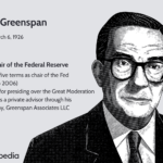
Alan Greenspan is an American economist who was the chair of the Board of Governors of the Federal Reserve (Fed), the United States’ central bank, from 1987 until 2006. In that role, he also served as the chair of the Federal Open Market Committee (FOMC), which is the Fed’s principal monetary policymaking committee that makes decisions on interest rates and managing the U.S. money supply.

Greenspan is best known for largely presiding over the Great Moderation, a period of relatively stable inflation and macroeconomic growth, that lasted from the mid-1980s to the financial crisis in 2007.

Early Life and Education

Alan Greenspan was born in New York City on March 6, 1926. He received his bachelor’s, master’s, and doctoral degrees in economics, all from New York University, as well as studying economics at Columbia University in the early 1950s under Arthur Burns, who would later serve two consecutive terms as chair of the Board of Governors of the Fed.

Greenspan’s first job, in 1948, was not in government but for a non-profit analyzing demand for steel, aluminum, and copper. After this, Greenspan ran an economic consulting firm in New York City, Townsend-Greenspan & Co., Inc., from 1954 to 1974 and 1977 to 1987. Greenspan began his career in the public sector in 1974 when he served as chair of the President’s Council of Economic Advisers (CEA) under President Gerald Ford.

In 1987, Greenspan became the 13th chair of the Fed, replacing Paul Volcker. President Ronald Reagan was the first to appoint Greenspan to the office, but three other presidents, George H.W. Bush, Bill Clinton, and George W. Bush, named him to four additional terms. His tenure as chair lasted for more than 18 years before he retired in 2006 to be replaced by Ben Bernanke. After leaving, he published his memoir, The Age of Turbulence, and began his own Washington DC-based consulting firm, Greenspan Associates LLC. 

Alan Greenspan was known as being adept at gaining consensus among Fed board members on policy issues and for serving during one of the most severe economic crises of the late 20th century, the aftermath of the stock market crash of 1987. After that crash, he advocated for sharply slashing interest rates to prevent the economy from sinking into a deep depression.

Alan Greenspan’s Policies and Actions

Greenspan presided over one of the most prosperous periods in American history—thanks in no small part, supporters feel, to his helming of the Fed. Still, some of his policies and actions were controversial, either at the time or in retrospect.

Views on Inflation

Early in his career, Greenspan developed a reputation for being hawkish on inflation, in part due to his advocacy for a return to the gold standard in monetary policy in the 1967 essay “Gold and Economic Freedom.” 

His allegedly “hawkish” stance was portrayed by early critics as a preference for sacrificing economic growth in exchange for preventing inflation. Greenspan eventually reversed those views as Fed chief; in a 1998 speech, he conceded that the new economy might not be as susceptible to inflation as he had first thought.

In practice, Greenspan’s supposedly hawkish approach was flexible, to say the least. He was clearly willing to risk inflation under conditions that could create a severe depression and certainly pursued a generally easy money policy relative to his predecessor, Paul Volcker. In particular, in the early 2000s, Greenspan presided over cutting interest rates to levels not seen in many decades.

Flip-Flop on Interest Rates

In 2000, Greenspan advocated reducing interest rates after the dot-com bubble burst. He did so again in 2001 after 9-11, the World Trade Center attack. Following 9-11, Greenspan led the FOMC to immediately reduce the Fed funds rate from 3.5% to 3%, and, in the following months, he worked toward lowering that rate to a record (at the time) low of 1.13% and holding it there for a full year.

Some criticized those rate cuts as having the potential to inflate asset price bubbles in the U.S. Greenspan’s pro-inflationary policies, particularly during this period, are today generally understood to have contributed to the U.S. housing bubble, subsequent subprime mortgage financial crisis, and the Great Recession, though this is of course disputed by Greenspan and his allies.

Encouraging Adjustable-Rate Mortgages

In a 2004 speech, Greenspan suggested more homeowners should consider taking out adjustable-rate mortgages (ARMs) where the interest rate adjusts itself to prevailing market interest rates. Under Greenspan’s tenure, interest rates subsequently rose as inflation accelerated. This increase reset many of those mortgages to much higher payments, creating even more distress for many homeowners and exacerbating the impact of that crisis.

The “Greenspan Put”

The “Greenspan put” was a monetary policy strategy popular during the 1990s and 2000s under Greenspan. Throughout his reign, he attempted to help support the U.S. economy by actively using the federal funds rate to aggressively lower interest rates to fight the deflation of asset price bubbles.

The Greenspan put created a substantial moral hazard in financial markets. Informed investors could expect the Fed to take predictable actions that would bailout investor’s losses, which distort the incentives of market participants. This created an environment where investors were encouraged to take excessive risk because Fed monetary policy tended to inherently limit their potential losses in the event of a market downturn in an analogous way to buying put options on the open market.

The Bottom Line

Like many other government officials, the success of Alan Greenspan’s five terms as Chair of the Fed will depend on who you ask. However, it is certainly true that Greenspan faced some massive challenges during his tenure, such as the 1987 stock market crash and the attacks on the World Trade Center.

Overall, Greenspan helped usher in a strong U.S. economy in the 1990s. Opinion on how much his actions caused the economic recession that began shortly after his term ended varies.

What Is the Alternative Minimum Tax?

An alternative minimum tax (AMT) places a floor on the percentage of taxes that a filer must pay to the government, no matter how many deductions or credits the filer may claim.

The United States currently has an alternative minimum tax for taxpayers who earn above certain income thresholds.

The AMT recalculates income tax after adding certain tax preference items back into adjusted gross income. It uses a separate set of rules to calculate taxable income after allowed deductions. Preferential deductions are added back into the taxpayer’s income to calculate their alternative minimum taxable income (AMTI), and then the AMT exemption is subtracted to determine the final taxable figure.

How the Alternative Minimum Tax Works

The difference between a taxpayer’s alternative minimum taxable income and his AMT exemption is taxed using the relevant rate schedule. This yields the tentative minimum tax (TMT).

If the tentative minimum tax is higher than the taxpayer’s regular tax liability for the year, then they pay the regular tax and the amount by which the tentative minimum tax exceeds the regular tax. In other words, the taxpayer pays the full tentative minimum tax.

There are two alternative minimum tax rates, 26% and 28%. For 2022, the 28% rate applies to excess alternative minimum taxable income of $206,100 or more for all taxpayers ($103,050 for married couples filing separate returns). For 2023, the 28% rate applies to excess alternative minimum taxable income of $220,700 or more for all taxpayers ($110,350 for married couples filing separate returns). The 26% rate applies to incomes up to those levels.

A taxpayer who has a high income and uses large tax breaks may owe a smaller percentage under the standard rules. If so, the taxpayer is obliged to recalculate the taxes owed under the alternative minimum tax system, which eliminates some of those tax breaks.

The taxpayer will owe whichever amount is higher.

AMT Exemption Amounts

For tax year 2022, the AMT exemption for single filers is $75,900. For married joint filers, the figure is $118,100. For tax year 2023, the figures are $81,300 for single filers and $126,500 for married joint filers.

Taxpayers have to complete Form 6251 to see whether they might owe AMT. First, they subtract the exemption amount from their income. If their AMT is less than the exemption, they do not have to pay AMT.

It’s important to note, though, that taxpayers with AMTI over a certain threshold do not qualify for the AMT exemption. For tax year 2022, the phase-out begins at $539,900 for single filers and $1,079,800 for couples filing jointly. For tax year 2023, the phase-out begins at $578,150 for single filers and $1,156,300.

Purpose of AMT

AMT is designed to prevent taxpayers from escaping their fair share of tax liability through tax breaks. However, in the past, the structure was not indexed to inflation or tax cuts. This can cause bracket creep, a condition in which middle-income taxpayers could be subject to this tax instead of just the wealthy taxpayers for whom AMT was invented. In 2012, however, Congress passed a law indexing the AMT exemption amount to inflation.

Calculating AMT

To determine if they owe AMT, individuals can use tax software that automatically does the calculation, or they can fill out IRS Form 6251. This form takes medical expenses, home mortgage interest, and several other miscellaneous deductions into account to help tax filers determine if their deductions are beyond an overall limit set by the IRS.

The form also requests information on certain types of income such as tax refunds, investment interest, and interest from private activity bonds, as well as numbers corresponding with capital gains or losses related to the disposition of property.

The IRS has specific formulas in place to determine which portion of this income and deductions the tax filers need to note on Form 6251. It uses another set of formulas to determine how these numbers lead to AMTI.

The Bottom Line

The Alternative Minimum Tax is an additional or parallel tax system in the U.S. that is designed to ensure that high-income individuals pay their fair share of taxes. Prior to the AMT, certain taxpayers paid little in the way of taxes, due to preferential treatment of certain income and expenses, or tax breaks.

What Is the Annual Equivalent Rate (AER)?

The annual equivalent rate (AER) is the interest rate for a savings account or investment product that has more than one compounding period. AER is calculated under the assumption that any interest paid is included in the principal payment’s balance and the next interest payment will be based on the slightly higher account balance.

The AER method means that interest can be compounded several times in a year, depending on the number of times that interest payments are made.

AER is also known as the effective annual interest rate or the annual percentage yield (APY).

The AER is the actual interest rate that an investor will earn for an investment, a loan, or another product, based on compounding. The AER reveals to investors what they can expect to return from an investment (the ROI)—the actual return of the investment based on compounding, which is more than the stated, or nominal, interest rate.

Assuming that interest is calculated—or compounded—more than once a year, the AER will be higher than the stated interest rate. The more compounding periods, the greater the difference between the two will be.

Formula for the AER


$\begin{aligned} &\text{Annual equivalent rate}=\left(1 + \frac{r}{n}\right)^n-1\\ &\textbf{where:}\\ &n=\text{The number of compounding periods (times per year interest is paid)}\\ &r = \text{The stated interest rate}\\ \end{aligned}$​Annual equivalent rate=(1+nr​)n−1where:n=The number of compounding periods (times per year interest is paid)r=The stated interest rate​

How to Calculate the AER

To calculate AER:

1. Divide the stated interest rate by the number of times a year that interest is paid (compounded) and add one.
2. Raise the result to the number of times a year that interest is paid (compounded)
3. Subtract one from the subsequent result.

The AER is displayed as a percentage (%).

Example of AER

Let’s look at AER in both savings accounts and bonds.

For a Savings Account

Assume an investor wishes to sell all the securities in their investment portfolio and place all the proceeds in a savings account. The investor is deciding between placing the proceeds in Bank A, Bank B, or Bank C, depending on the highest rate offered. Bank A has a quoted interest rate of 3.7% that pays interest on an annual basis. Bank B has a quoted interest rate of 3.65% that pays interest quarterly, and Bank C has a quoted interest rate of 3.7% that pays interest semi-annually.

Therefore, Bank A would have an annual equivalent rate of 3.7%, or (1 + (0.037 / 1))¹ – 1. Bank B has an AER of 3.7% = (1 + (0.0365 / 4))⁴ – 1, which is equivalent to that of Bank A even though Bank B is compounded quarterly. It would thus make no difference to the investor if they placed their cash in Bank A or Bank B.

On the other hand, Bank C has the same interest rate as Bank A, but Bank C pays interest semi-annually. Consequently, Bank C has an AER of 3.73%, which is more attractive than the other two banks’ AER. The calculation is (1 + (0.037 / 2))² – 1 = 3.73%.

With a Bond

Let’s now consider a bond issued by General Electric. As of March 2019, General Electric offers a noncallable semiannual coupon with a 4% coupon rate expiring Dec. 15, 2023. The nominal, or stated rate, of the bond, is 8%—or the 4% coupon rate times two annual coupons. However, the annual equivalent rate is higher, given the fact that interest is paid twice a year. The AER of the bond is calculated as (1+ (0.04 / 2 ))² – 1 = 8.16%.

Annual Equivalent Rate vs. Stated Interest

While the stated interest rate doesn’t account for compounding, the AER does. The stated rate will generally be lower than AER if there’s more than one compounding period. AER is used to determine which banks offer better rates and which investments might be attractive.

Advantages and Disadvantages of the AER

The primary advantage of AER is that it is the real rate of interest because it accounts for the effects of compounding. In addition, it is an important tool for investors because it helps them evaluate bonds, loans, or accounts to understand their real return on investment (ROI).

Unfortunately, when investors are evaluating different investment options, the AER is usually not stated. Investors must do the work of calculating the figure themselves. It’s also important to keep in mind that AER doesn’t include any fees that might be tied to purchasing or selling the investment. Also, compounding itself has limitations, with the maximum possible rate being continuous compounding.

Special Considerations

AER is one of the various ways to calculate interest on interest, which is called compounding. Compounding refers to earning or paying interest on previous interest, which is added to the principal sum of a deposit or loan. Compounding allows investors to boost their returns because they can accrue additional profit based on the interest they’ve already earned.

One of Warren Buffett’s famous quotes is, “My wealth has come from a combination of living in America, some lucky genes, and compound interest.” Albert Einstein reportedly referred to compound interest as mankind’s greatest invention. 

When you are borrowing money (in the form of loans), you want to minimize the effects of compounding. On the other hand, all investors want to maximize compounding on their investments. Many financial institutions will quote interest rates that use compounding principles to their advantage. As a consumer, it is important to understand AER so you can determine the interest rate you are really getting.

What is Activity-Based Budgeting (ABB)?

Activity-based budgeting (ABB) is a system that records, researches, and analyzes activities that lead to costs for a company. Every activity in an organization that incurs a cost is scrutinized for potential ways to create efficiencies. Budgets are then developed based on these results.

Activity-based budgeting (ABB) is more rigorous than traditional budgeting processes, which tend to merely adjust previous budgets to account for inflation or business development.

How Activity-Based Budgeting (ABB) Works

Keeping costs to a minimum is a crucial part of business management. When done effectively and not too excessively, companies should be able to maintain and keep growing their revenues, while squeezing out higher profits from them.

Using activity-based budgeting (ABB) can help companies to reduce the activity levels required to generate sales. Eliminating unnecessary costs should boost profitability.

The activity-based budgeting (ABB) process is broken down into three steps.

1. Identify relevant activities. These cost drivers are the items responsible for incurring revenue or expenses for the company.
2. Determine the number of units related to each activity. This number is the baseline for calculations.
3. Delineate the cost per unit of activity and multiply that result by the activity level.

Activity-Based Budgeting (ABB) Vs. Traditional Budgeting Processes

Activity-based budgeting (ABB) is an alternative budgeting practice. Traditional methods are more simplistic, adjusting prior period budgets to account for inflation or revenue growth. Rather than using past budgets to calculate how much a firm will spend in the current year, activity-based budgeting (ABB) digs deeper.

Activity-based budgeting (ABB) is not necessary for all companies. For example, established firms that experience minimal change typically find that applying a flat rate to data from the previous year to reflect business growth and inflation is sufficient.

In contrast, newer companies without access to historical budgeting information cannot consider this an option. Activity-based budgeting (ABB) is also likely to be implemented by firms undergoing material changes, such as those with new subsidiaries, significant customers, business locations, or products. In these types of cases, historical information may no longer be a useful basis for future budgeting.

Example of Activity-Based Budgeting

Company A anticipates receiving 50,000 sales orders in the upcoming year, with each single order costing $2 to process. Therefore, the activity-based budget (ABB) for the expenses relating to processing sales orders for the upcoming year is $100,000 ($50,000 * $2). 

This figure may be compared to a traditional approach to budgeting. If last year’s budget called for $80,000 of sales order processing expenses and sales were expected to grow 10%, only $88,000 ($80,000 + ($80,000 * 10%)) is budgeted.

Advantages and Disadvantages of Activity-Based Budgeting

Activity-based budgeting (ABB) systems allow for more control over the budgeting process. Revenue and expense planning occurs at a precise level that provides useful details regarding projections. ABB allows for management to have increased control over the budgeting process and to align the budget with overall company goals.

Unfortunately, these benefits come at a cost. Activity-based budgeting (ABB) is more expensive to implement and maintain than traditional budgeting techniques and more time consuming as well. Moreover, ABB systems need additional assumptions and insight from management, which can, on occasion, result in potential budgeting inaccuracies.